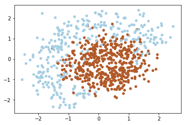
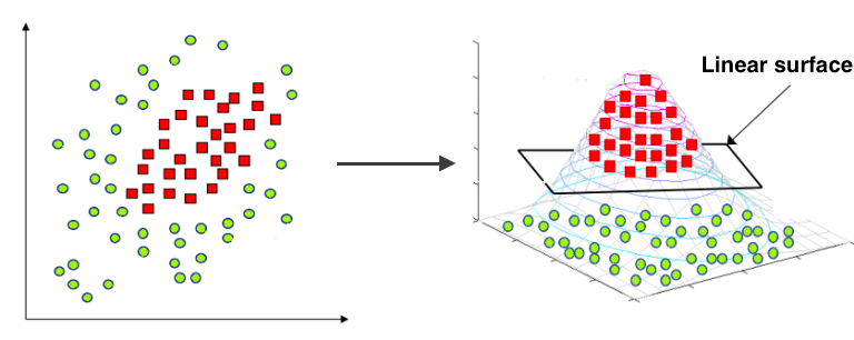
As you can notice the data above isn’t linearly separable. Since that we should add features (or use non-linear model). Note that decision line between two classes have form of circle, since that we can add quadratic features to make the problem linearly separable. The idea under this displayed on image below:
Common under-fitting example for linear models:
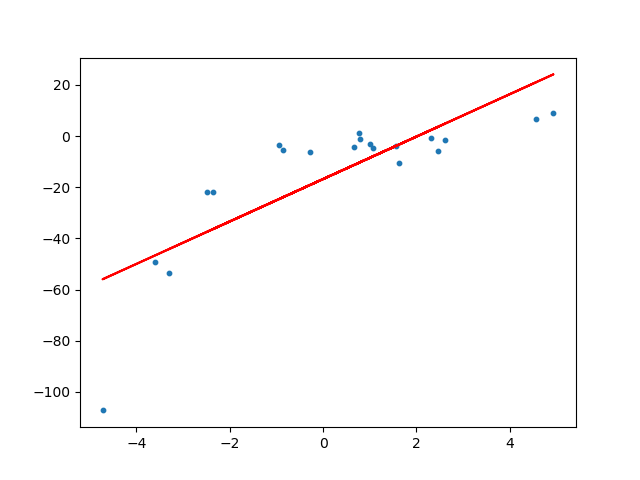
To overcome under-fitting, we need to increase the complexity of the model.
To generate a higher order equation we can add powers of the original features as new features, in other words, you can cleverly transform your input data in order to fit a quadratic curve with a linear regression model. Consider the 2D case above.
The linear model:
can be transformed to:
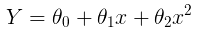
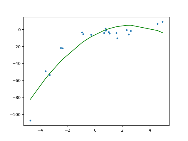
This is still considered to be linear model as the coefficients/weights associated with the features are still linear. x² is only a feature. However the curve that we are fitting is quadratic in nature.
Fitting a linear regression model on the transformed features gives the below plot.
def expand(X):
    """
    Adds quadratic features.
    This expansion allows your linear model to make non-linear separation.

    For each sample (row in matrix), compute an expanded row:
    [feature0, feature1, feature0^2, feature1^2, feature0*feature1, 1]

    :param X: matrix of features, shape [n_samples,2]
    :returns: expanded features of shape [n_samples,6]
    """
    X_expanded = np.zeros((X.shape[0], 6))

    expanded = np.apply_along_axis(row_expander, axis=1, arr=X)

    return expanded

def row_expander(row):

    feature0 = row[0]
    feature1 = row[1]

    expanded_row = np.array([feature0, feature1, pow(feature0,2), pow(feature1,2), feature0*feature1, 1])

    return expanded_row