HOW IT WORKS

Convolutional neural networks (CNNs) are a biologically-inspired variation of the multilayer perceptrons (MLPs).

Neurons in CNNs share weights unlike in MLPs where each neuron has a separate weight vector. This sharing of weights ends up reducing the overall number of trainable weights hence introducing sparsity.

Utilizing the weights sharing strategy, neurons are able to perform convolutions on the data with the convolution filter being formed by the weights. This is then followed by a pooling operation which as a form of non-linear down-sampling, progressively reduces the spatial size of the representation thus reducing the amount of computation and parameters in the network.

2D CONVOLUTON

A convolution sweeps the window through images then calculates its input and filter dot product pixel values. This allows convolution to emphasize the relevant features.

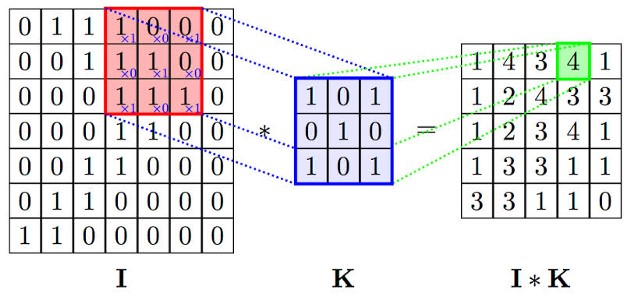
With this computation, you detect a particular feature from the input image and produce** feature maps **(convolved features) which emphasizes the important features. These convolved features will always change depending on the filter values affected by the gradient descent to minimize prediction loss.

FOWARD PROPAGATION

To perform a convolution operation, the kernel is flipped 180º and slid across the input feature map in equal and finite strides. At each location, the product between each element of the kernel and the input input feature map element it overlaps is computed and the results summed up to obtain the output at that current location.

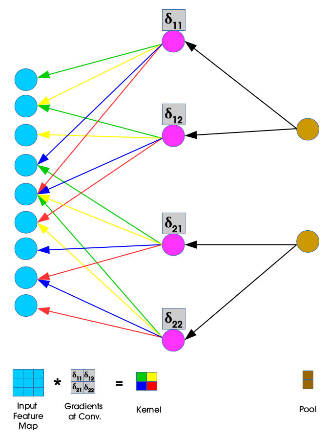
This procedure is repeated using different kernels to form as many output feature maps as desired. The concept of weight sharing is used as demonstrated in the diagram below:

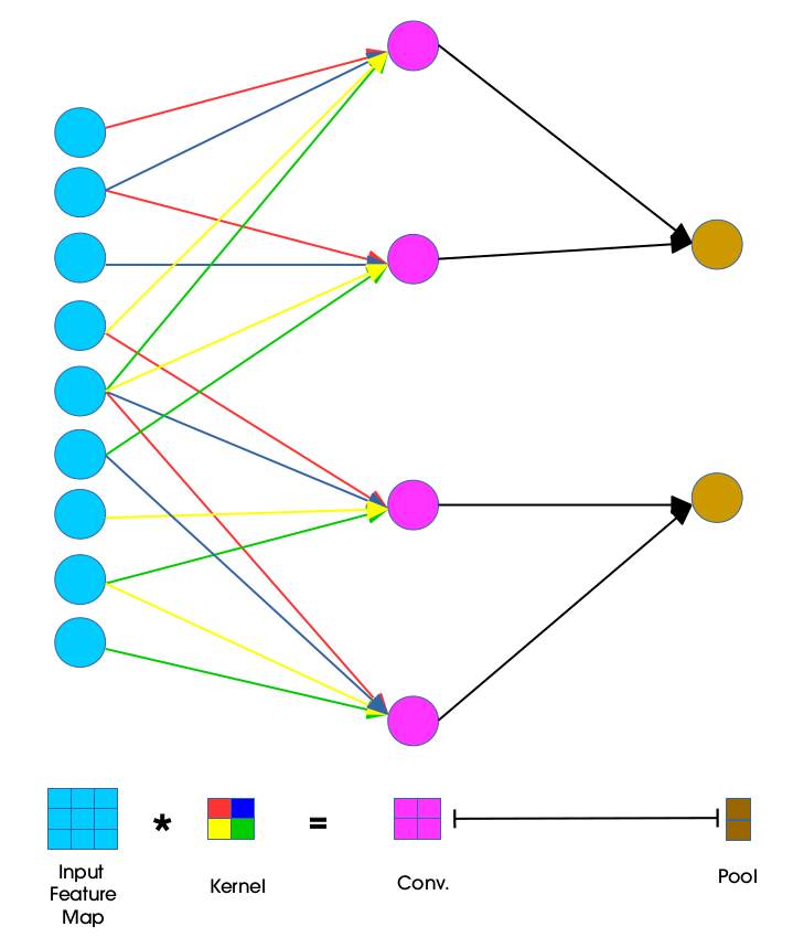
Units in convolutional layer illustrated above have receptive fields of size 4 in the input feature map and are thus only connected to 4 adjacent neurons in the input layer. This is the idea of sparse connectivity in CNNs where there exists local connectivity pattern between neurons in adjacent layers.

The color codes of the weights joining the input layer to the convolutional layer show how the kernel weights are distributed (shared) amongst neurons in the adjacent layers. Weights of the same color are constrained to be identical.

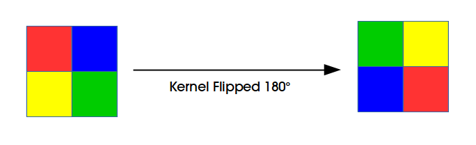
The convolution process here is usually expressed as a cross-correlation but with a flipped kernel. In the diagram below we illustrate a kernel that has been flipped both horizontally and vertically:

LOSS (ERROR)

For a total of P predictions, the predicted network outputs yp and their corresponding targeted values tptp the the mean squared error is given by:

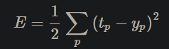
Learning will be achieved by adjusting the weights such that yp is as close as possible or equals to corresponding tp. In the classical backpropagation algorithm, the weights are changed according to the gradient descent direction of an error surface E.

BACKPROPAGATION

For backpropagation there are two updates performed, for the weights and the deltas. Lets begin with the weight update. We are looking to compute:

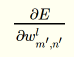
which can be interpreted as the measurement of how the change in a single pixel wm′,n′ in the weight kernel affects the loss function E.

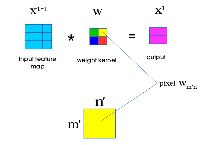
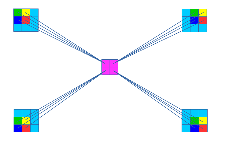
During forward propagation, the convolution operation ensures that the yellow pixel wm′,n′ in the weight kernel makes a contribution in all the products (between each element of the weight kernel and the input feature map element it overlaps). This means that pixel wm′,n′ will eventually affect all the elements in the output feature map.

Convolution between the input feature map of dimension H × W and the weight kernel of dimension k1 × k2 produces an output feature map of size (H − k1 + 1) by (W − k2 + 1). The gradient component for the individual weights can be obtained by applying the chain rule in the following way:

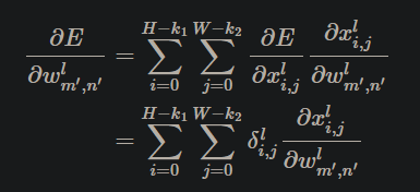
After some math magic, it give us:

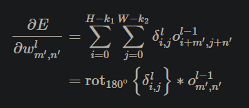
The dual summation is as a result of weight sharing in the network (same weight kernel is slid over all of the input feature map during convolution). The summations represents a collection of all the gradients δl_i,j coming from all the outputs in layer L.

Obtaining gradients w.r.t to the filter maps, we have a cross-correlation which is transformed to a convolution by “flipping” the delta matrix δl_i,j (horizontally and vertically) the same way we flipped the filters during the forward propagation.

The convolution operation used to obtain the new set of weights as is shown below:

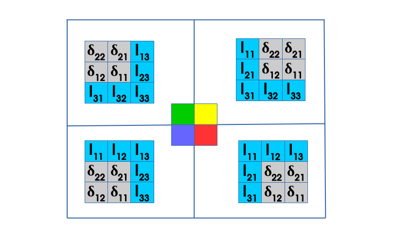
During the reconstruction process, the deltas (δ11, δ12, δ21, δ22) are used. These deltas are provided by an equation of the form:

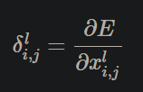
Which can be interpreted as the measurement of how the change in a single pixel xi′,j′ in the input feature map affects the loss function E.

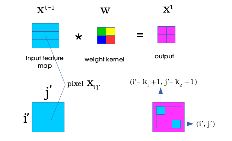
From the diagram above, we can see that region in the output affected by pixel xi′,j′ from the input is the region in the output bounded by the dashed lines where the top left corner pixel is given by (i′ − k1 + 1, j′ − k2 + 1) and the bottom right corner pixel is given by (i′,j′).

Using chain rule and introducing sums give us the following equation:

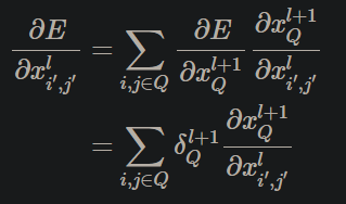
Again, after some math magic, we ended up with:

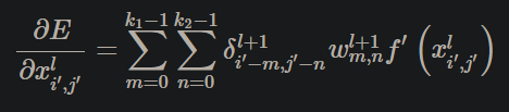
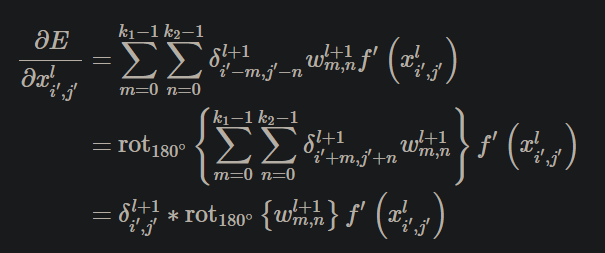
For backpropagation, we make use of the flipped kernel and as a result we will now have a convolution that is expressed as a cross-correlation with a flipped kernel: