
Consider a scenario where we need to classify whether an email is spam or not. If we use linear regression for this problem, there is a need for setting up a threshold based on which classification can be done. Say if the actual class is malignant, predicted continuous value 0.4 and the threshold value is 0.5, the data point will be classified as not malignant which can lead to serious consequence in real time.
From this example, it can be inferred that linear regression is not suitable for classification problem. Linear regression is unbounded, and this brings logistic regression into picture. Their value strictly ranges from 0 to 1.
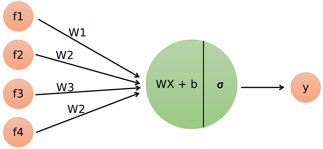
Problem Formulation:
- Output = 0 or 1
- Hypothesis ⇒
Z = WX + B - hΘ(x) = sigmoid (Z)
Given the sigmoid function:
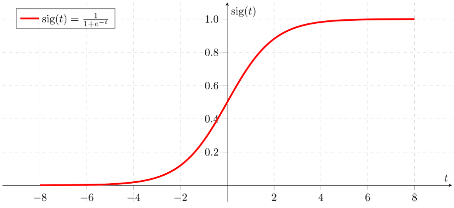
If ‘Z’ goes to infinity, Y(predicted) will become 1 and if ‘Z’ goes to negative infinity, Y(predicted) will become 0.
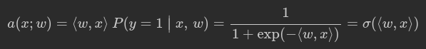
The output from the hypothesis is the estimated probability. This is used to infer how confident can predicted value be actual value when given an input X.
## LOSS
To classify objects we will obtain probability of object belongs to class ‘1’. To predict probability we will use output of linear model and logistic function:
def probability(X, w):
    """
    Given input features and weights
    return predicted probabilities of y==1 given x, P(y=1|x), see description above

    Don't forget to use expand(X) function (where necessary) in this and subsequent functions.

    :param X: feature matrix X of shape [n_samples,6] (expanded)
    :param w: weight vector w of shape [6] for each of the expanded features
    :returns: an array of predicted probabilities in [0,1] interval.
    """

    return 1 / (1 + np.exp(-np.dot(w, X.T)))
In logistic regression the optimal parameters w are found by cross-entropy minimization:

Where m is the number of samples, x**ᵢ is the i-th training example, *yᵢ *its class (i.e. either 0 or 1), σ(z) is the logistic function and w is the vector of parameters of the model.
For logistic regression, it is a convex function. As such, any minimum is a global minimum.
def compute_loss(X, y, w):
    """
    Given feature matrix X [n_samples,6], target vector [n_samples] of 1/0,
    and weight vector w [6], compute scalar loss function L using formula above.
    Keep in mind that our loss is averaged over all samples (rows) in X.
    """

    l = X.shape[0]
    prob = probability(X, w)

    return -1/l * np.sum(y * np.log(prob) + (1 - y) * np.log(1 - prob))
To train the model with gradient descent, we should compute gradients. To be specific, we need a derivative of loss function over each weight.
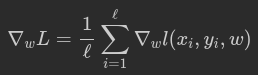
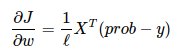
def compute_grad(X, y, w):
    """
    Given feature matrix X [n_samples,6], target vector [n_samples] of 1/0,
    and weight vector w [6], compute vector [6] of derivatives of L over each weights.
    Keep in mind that our loss is averaged over all samples (rows) in X.
    """

    l = X.shape[0]
    prob = probability(X, w)

    return 1/l * np.dot(X.T, (prob - y))
https://towardsdatascience.com/binary-cross-entropy-and-logistic-regression-bf7098e75559
## TRAINING
Stochastic Gradient Descent just takes a random example on each iteration, and calculates a gradient of the loss on it and makes a step:
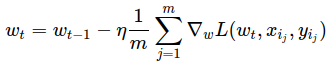
# please use np.random.seed(42), eta=0.1, n_iter=100 and batch_size=4 for deterministic results

np.random.seed(42)
w = np.array([0, 0, 0, 0, 0, 1])

eta = 0.1 # learning rate

n_iter = 100
batch_size = 4
loss = np.zeros(n_iter)
plt.figure(figsize=(12, 5))

for i in range(n_iter):
    ind = np.random.choice(X_expanded.shape[0], batch_size)
    loss[i] = compute_loss(X_expanded, y, w)
    if i % 10 == 0:
        visualize(X_expanded[ind, :], y[ind], w, loss)

    w = w - eta * compute_grad(X_expanded, y, w)

visualize(X, y, w, loss)
plt.clf()