LOAD DATASET
Let’s load an images dataset, that will be used for train and test. This dataset is composed by 60000 RGB images (32 x 32):
from keras.datasets import cifar10
(x_train, y_train), (x_test, y_test) = cifar10.load_data()
print("Train samples:", x_train.shape, y_train.shape)
print("Test samples:", x_test.shape, y_test.shape)
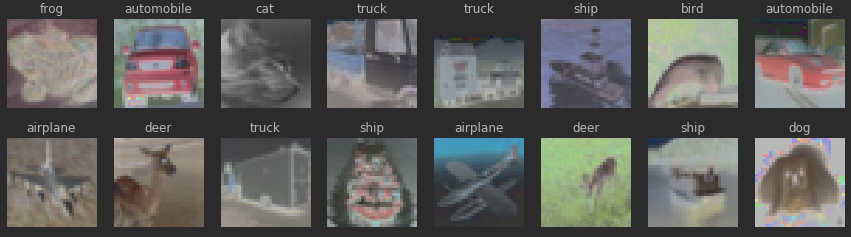
NUM_CLASSES = 10
cifar10_classes = ["airplane", "automobile", "bird", "cat", "deer",
"dog", "frog", "horse", "ship", "truck"]
cols = 8
rows = 2
fig = plt.figure(figsize=(2 * cols - 1, 2.5 * rows - 1))
for i in range(cols):
for j in range(rows):
random_index = np.random.randint(0, len(y_train))
ax = fig.add_subplot(rows, cols, i * rows + j + 1)
ax.grid('off')
ax.axis('off')
ax.imshow(x_train[random_index, :])
ax.set_title(cifar10_classes[y_train[random_index, 0]])
plt.show()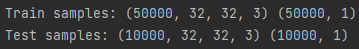
PREPARE DARA
We need to normalize the inputs (images) using:
Here we are dividing each feature (pixel) value by the standard deviation. Subtracting the mean centers the input to 0, and dividing by the standard deviation makes any scaled feature value the number of standard deviations away from the mean.
Consider how a neural network learns its weights. CNNs learn by continually adding gradient error vectors (multiplied by a learning rate) computed from backpropagation to various weight matrices throughout the network as training examples are passed through.
The thing to notice here is the “multiplied by a learning rate”.
If we didn’t scale our input training vectors, the ranges of our distributions of feature values would likely be different for each feature, and thus the learning rate would cause corrections in each dimension that would differ (proportionally speaking) from one another. We might be over compensating a correction in one weight dimension while undercompensating in another.
# normalize inputs
x_train2 = x_train / 255 - 0.5
x_test2 = x_test / 255 - 0.5


# We need to convert class labels to one-hot encoded vectors. Use __keras.utils.to_categorical__.
# convert class labels to one-hot encoded, should have shape (?, NUM_CLASSES)
y_train2 = keras.utils.to_categorical(y_train, num_classes=NUM_CLASSES)
y_test2 = keras.utils.to_categorical(y_test, num_classes=NUM_CLASSES)


print(y_train2.shape)
print(y_test2.shape)
DEFINE CNN ARCHITECTURE
# import necessary building blocks
from keras.models import Sequential
from keras.layers import Conv2D, MaxPooling2D, Flatten, Dense, Activation, Dropout
from keras.layers.advanced_activations import LeakyReLU
You need to define a model which takes **(None, 32, 32, 3)** input and predicts **(None, 10)** output with probabilities for all classes. **None** in shapes stands for batch dimension.
Simple feed-forward networks in Keras can be defined in the following way:
model = Sequential()  # start feed-forward model definition
model.add(Conv2D(..., input_shape=(32, 32, 3)))  # first layer needs to define "input_shape"

...  # here comes a bunch of convolutional, pooling and dropout layers

model.add(Dense(NUM_CLASSES))  # the last layer with neuron for each class
model.add(Activation("softmax"))  # output probabilities
The recipe:
- Stack 4 convolutional layers with kernel size (3, 3) with growing number of filters (16, 32, 32, 64), use “same” padding.
- Add 2x2 pooling layer after every 2 convolutional layers (conv-conv-pool scheme).
- Use LeakyReLU activation with recommended parameter 0.1 for all layers that need it (after convolutional and dense layers)
- Add a dense layer with 256 neurons and a second dense layer with 10 neurons for classes. Remember to use Flatten layer before first dense layer to reshape input volume into a flat vector!
- Add Dropout after every pooling layer (0.25) and between dense layers (0.5).
def make_model():
    """
    Define your model architecture here.
    Returns `Sequential` model.
    """
    model = Sequential()

    # CONV 1
    # first layer needs to define "input_shape"
    model.add(Conv2D(16, (3, 3), strides = (1, 1), padding="same", name = 'conv1', input_shape=(32, 32, 3)))
    model.add(LeakyReLU(0.1))

    # CONV 2
    model.add(Conv2D(32, (3, 3), strides = (1, 1), padding="same", name = 'conv2'))
    model.add(LeakyReLU(0.1))

    # MaxPooling2D 1
    model.add(MaxPooling2D((2, 2), name='max_pool_1'))

    # Dropout
    model.add(Dropout(0.25, noise_shape=None, seed=0))

    # CONV 3
    model.add(Conv2D(32, (3, 3), strides = (1, 1), padding="same", name = 'conv3'))
    model.add(LeakyReLU(0.1))

    # CONV 4
    model.add(Conv2D(64, (3, 3), strides = (1, 1), padding="same", name = 'conv4'))
    model.add(LeakyReLU(0.1))

    # MaxPooling2D 1
    model.add(MaxPooling2D((2, 2), name='max_pool_2'))

    # Dropout
    model.add(Dropout(0.25, noise_shape=None, seed=0))

    # Flatten
    model.add(Flatten())

    # FC
    model.add(Dense(256, name='fc1'))
    model.add(Dropout(0.5, noise_shape=None, seed=0))

    # FC
    model.add(Dense(NUM_CLASSES))  # the last layer with neuron for each class
    model.add(Activation("softmax"))  # output probabilities

    return model
Running model.summary() will show the complete assembled model architecture:
# describe model
s = reset_tf_session()  # clear default graph
model = make_model()
model.summary()
_________________________________________________________________
Layer (type) Output Shape Param #
=================================================================
conv1 (Conv2D) (None, 32, 32, 16) 448
_________________________________________________________________
leaky_re_lu_1 (LeakyReLU) (None, 32, 32, 16) 0
_________________________________________________________________
conv2 (Conv2D) (None, 32, 32, 32) 4640
_________________________________________________________________
leaky_re_lu_2 (LeakyReLU) (None, 32, 32, 32) 0
_________________________________________________________________
max_pool_1 (MaxPooling2D) (None, 16, 16, 32) 0
_________________________________________________________________
dropout_1 (Dropout) (None, 16, 16, 32) 0
_________________________________________________________________
conv3 (Conv2D) (None, 16, 16, 32) 9248
_________________________________________________________________
leaky_re_lu_3 (LeakyReLU) (None, 16, 16, 32) 0
_________________________________________________________________
conv4 (Conv2D) (None, 16, 16, 64) 18496
_________________________________________________________________
leaky_re_lu_4 (LeakyReLU) (None, 16, 16, 64) 0
_________________________________________________________________
max_pool_2 (MaxPooling2D) (None, 8, 8, 64) 0
_________________________________________________________________
dropout_2 (Dropout) (None, 8, 8, 64) 0
_________________________________________________________________
flatten_1 (Flatten) (None, 4096) 0
_________________________________________________________________
fc1 (Dense) (None, 256) 1048832
_________________________________________________________________
dropout_3 (Dropout) (None, 256) 0
_________________________________________________________________
dense_1 (Dense) (None, 10) 2570
_________________________________________________________________
activation_1 (Activation) (None, 10) 0
=================================================================
Total params: 1,084,234
Trainable params: 1,084,234
Non-trainable params: 0
_________________________________________________________________TRAIN MODEL
INIT_LR = 5e-3  # initial learning rate
BATCH_SIZE = 32
EPOCHS = 10

s = reset_tf_session()  # clear default graph
# don't call K.set_learning_phase() !!! (otherwise will enable dropout in train/test simultaneously)
model = make_model()  # define our model

# prepare model for fitting (loss, optimizer, etc)
model.compile(
    loss='categorical_crossentropy',  # we train 10-way classification
    optimizer=keras.optimizers.adamax(lr=INIT_LR),  # for SGD
    metrics=['accuracy']  # report accuracy during training
)


## CALLBACKS
# scheduler of learning rate (decay with epochs)
def lr_scheduler(epoch):
    return INIT_LR * 0.9 ** epoch

# callback for printing of actual learning rate used by optimizer
class LrHistory(keras.callbacks.Callback):
    def on_epoch_begin(self, epoch, logs={}):
        print("Learning rate:", K.get_value(model.optimizer.lr))
# we will save model checkpoints to continue training in case of kernel death
model_filename = 'cifar.{0:03d}.hdf5'
last_finished_epoch = None
#### uncomment below to continue training from model checkpoint
#### fill `last_finished_epoch` with your latest finished epoch
from keras.models import load_model
s = reset_tf_session()
last_finished_epoch = 8
model = load_model(model_filename.format(last_finished_epoch))# fit model
model.fit(
x_train2, y_train2, # prepared data
batch_size=BATCH_SIZE,
epochs=EPOCHS,
callbacks=[keras.callbacks.LearningRateScheduler(lr_scheduler),
LrHistory(),
keras_utils.TqdmProgressCallback(),
keras_utils.ModelSaveCallback(model_filename)],
validation_data=(x_test2, y_test2),
shuffle=True,
verbose=0,
initial_epoch=last_finished_epoch or 0
)
# save weights to file
model.save_weights("weights.h5")
# load weights from file (can call without model.fit)
model.load_weights("weights.h5")EVALUATE MODEL
# make test predictions
y_pred_test = model.predict_proba(x_test2)
y_pred_test_classes = np.argmax(y_pred_test, axis=1)
y_pred_test_max_probas = np.max(y_pred_test, axis=1)
# confusion matrix and accuracy
from sklearn.metrics import confusion_matrix, accuracy_score
plt.figure(figsize=(7, 6))
plt.title('Confusion matrix', fontsize=16)
plt.imshow(confusion_matrix(y_test, y_pred_test_classes))
plt.xticks(np.arange(10), cifar10_classes, rotation=45, fontsize=12)
plt.yticks(np.arange(10), cifar10_classes, fontsize=12)
plt.colorbar()
plt.show()
print("Test accuracy:", accuracy_score(y_test, y_pred_test_classes))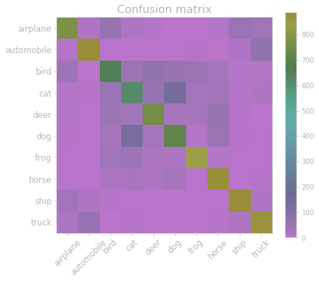
# inspect preditions
cols = 8
rows = 2

fig = plt.figure(figsize=(2 * cols - 1, 3 * rows - 1))

for i in range(cols):

    for j in range(rows):

        random_index = np.random.randint(0, len(y_test))

        ax = fig.add_subplot(rows, cols, i * rows + j + 1)

        ax.grid('off')
        ax.axis('off')

        ax.imshow(x_test[random_index, :])
        pred_label = cifar10_classes[y_pred_test_classes[random_index]]
        pred_proba = y_pred_test_max_probas[random_index]
        true_label = cifar10_classes[y_test[random_index, 0]]
        ax.set_title("pred: {}\nscore: {:.3}\ntrue: {}".format(
               pred_label, pred_proba, true_label
        ))

plt.show()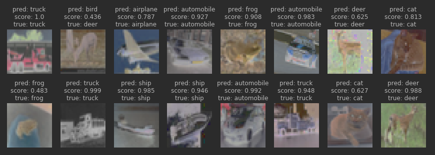
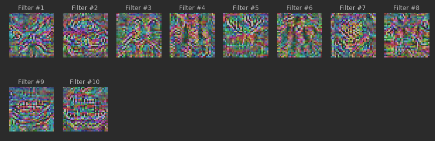
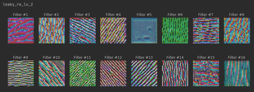
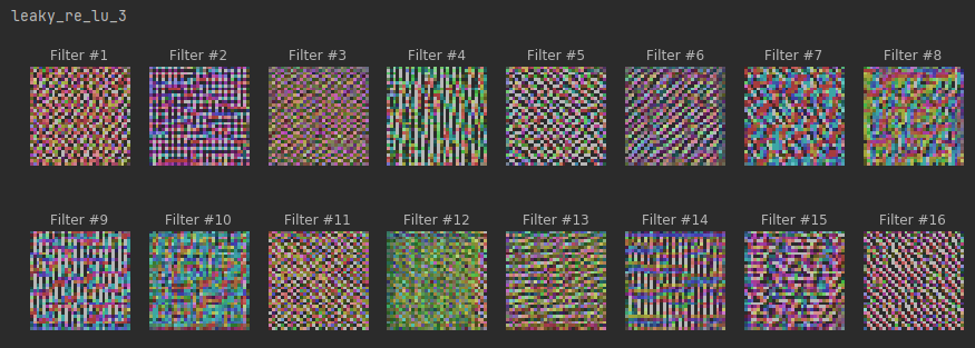
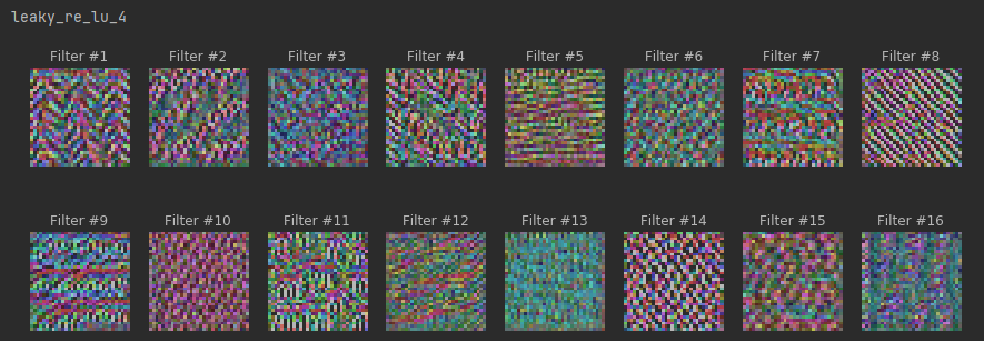
VISUALIZE MAXIMUM STIMULI
s = reset_tf_session()  # clear default graph
K.set_learning_phase(0)  # disable dropout
model = make_model()
model.load_weights("weights.h5")  # that were saved after model.fit

def find_maximum_stimuli(layer_name, is_conv, filter_index, model, iterations=20, step=1., verbose=True):

    def image_values_to_rgb(x):
        # normalize x: center on 0 (np.mean(x_train2)), ensure std is 0.25 (np.std(x_train2))
        # so that it looks like a normalized image input for our network
        x = (x - np.mean(x_train2)) / np.std(x_train2)

        # do reverse normalization to RGB values: x = (x_norm + 0.5) * 255
        x = (x + 0.5) * 255

        # clip values to [0, 255] and convert to bytes
        x = np.clip(x, 0, 255).astype('uint8')
        return x

    # this is the placeholder for the input image
    input_img = model.input
    img_width, img_height = input_img.shape.as_list()[1:3]

    # find the layer output by name
    layer_output = list(filter(lambda x: x.name == layer_name, model.layers))[0].output

    # we build a loss function that maximizes the activation
    # of the filter_index filter of the layer considered
    if is_conv:
        # mean over feature map values for convolutional layer
        loss = K.mean(layer_output[:, :, :, filter_index])
    else:
        loss = K.mean(layer_output[:, filter_index])

    # we compute the gradient of the loss wrt input image
    grads = K.gradients(loss, input_img)[0]  # [0] because of the batch dimension!

    # normalization trick: we normalize the gradient
    grads = grads / (K.sqrt(K.sum(K.square(grads))) + 1e-10)

    # this function returns the loss and grads given the input picture
    iterate = K.function([input_img], [loss, grads])

    # we start from a gray image with some random noise
    input_img_data = np.random.random((1, img_width, img_height, 3))
    input_img_data = (input_img_data - 0.5) * (0.1 if is_conv else 0.001)

    # we run gradient ascent
    for i in range(iterations):
        loss_value, grads_value = iterate([input_img_data])
        input_img_data += grads_value * step
        if verbose:
            print('Current loss value:', loss_value)

    # decode the resulting input image
    img = image_values_to_rgb(input_img_data[0])

    return img, loss_value
# sample maximum stimuli
def plot_filters_stimuli(layer_name, is_conv, model, iterations=20, step=1., verbose=False):
cols = 8
rows = 2
filter_index = 0
max_filter_index = list(filter(lambda x: x.name == layer_name, model.layers))[0].output.shape.as_list()[-1] - 1
fig = plt.figure(figsize=(2 * cols - 1, 3 * rows - 1))
for i in range(cols):
for j in range(rows):
if filter_index <= max_filter_index:
ax = fig.add_subplot(rows, cols, i * rows + j + 1)
ax.grid('off')
ax.axis('off')
loss = -1e20
while loss < 0 and filter_index <= max_filter_index:
stimuli, loss = find_maximum_stimuli(layer_name, is_conv, filter_index, model,
iterations, step, verbose=verbose)
filter_index += 1
if loss > 0:
ax.imshow(stimuli)
ax.set_title("Filter #{}".format(filter_index))
plt.show()# maximum stimuli for convolutional neurons
conv_activation_layers = []
for layer in model.layers:
if isinstance(layer, LeakyReLU):
prev_layer = layer.inbound_nodes[0].inbound_layers[0]
if isinstance(prev_layer, Conv2D):
conv_activation_layers.append(layer)
for layer in conv_activation_layers:
print(layer.name)
plot_filters_stimuli(layer_name=layer.name, is_conv=True, model=model)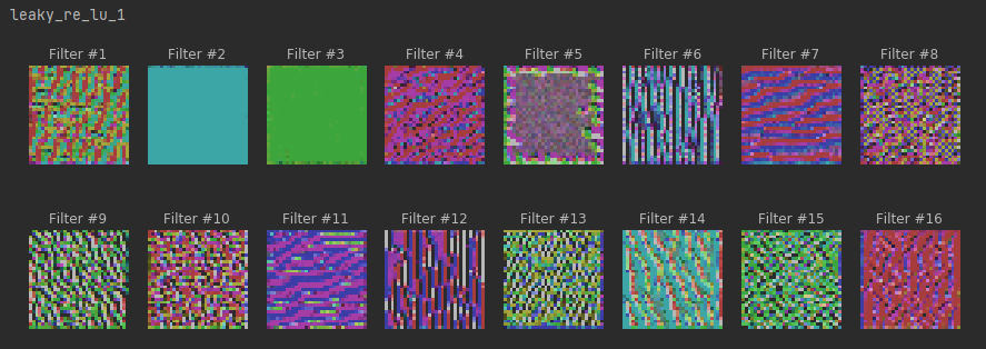
# maximum stimuli for last dense layer
last_dense_layer = list(filter(lambda x: isinstance(x, Dense), model.layers))[-1]
plot_filters_stimuli(layer_name=last_dense_layer.name, is_conv=False,
                     iterations=200, step=0.1, model=model)