NN from Scratch

LAYERS

Every layer will have a forward pass and backpass implementation. Let’s create a main class layer which can do a forward pass .forward() and Backward pass .backward().

class Layer:
    """
    A building block. Each layer is capable of performing two things:
    
    - Process input to get output: output = layer.forward(input)
    
    - Propagate gradients through itself: grad_input = layer.backward(input, grad_output)
    
    Some layers also have learnable parameters which they update during layer.backward.
    """
    def __init__(self):
        """Here you can initialize layer parameters (if any) and auxiliary stuff."""
        # A dummy layer does nothing
        pass
    
    def forward(self, input):
        """
        Takes input data of shape [batch, input_units], returns output data [batch, output_units]
        """
        # A dummy layer just returns whatever it gets as input.
        return input
 
    def backward(self, input, grad_output):
        """
        Performs a backpropagation step through the layer, with respect to the given input.
        
        To compute loss gradients w.r.t input, you need to apply chain rule (backprop):
        
        d loss / d x  = (d loss / d layer) * (d layer / d x)
        
        Luckily, you already receive d loss / d layer as input, so you only need to multiply it by d layer / d x.
        
        If your layer has parameters (e.g. dense layer), you also need to update them here using d loss / d layer
        """
        # The gradient of a dummy layer is precisely grad_output, but we'll write it more explicitly
        num_units = input.shape[1]
        
        d_layer_d_input = np.eye(num_units)
        
        return np.dot(grad_output, d_layer_d_input) # chain rule

This is the simplest layer you can get: it simply applies a nonlinearity to each element of your network.

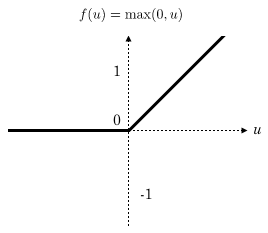
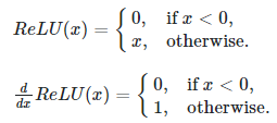
On backward (backpropagation stuff), using ReLU function f(x)=max(0,x). if x<=0 then f(x)=0, else f(x)=x. In the first case, when x<0 so the derivative of f(x) with respect to x gives result f'(x)=0. In the second case, it’s clear to compute f'(x)=1.

class ReLU(Layer):
 
    def __init__(self):
        """ReLU layer simply applies elementwise rectified linear unit to all inputs"""
        pass
    
    def forward(self, input):
        """Apply elementwise ReLU to [batch, input_units] matrix"""
        # <your code. Try np.maximum>
        return np.maximum(0, input)
    
    def backward(self, input, grad_output):
        """Compute gradient of loss w.r.t. ReLU input"""
        relu_grad = input > 0
        return grad_output * relu_grad

Unlike nonlinearity, a dense layer actually has something to learn. A dense layer applies affine transformation. In a vectorized form, it can be described as:

$f (X) = W \cdot X + b ⃗$

Where:

X is an object-feature matrix of shape [batch_size, num_features],
W is a weight matrix [num_features, num_outputs]
and b is a vector of num_outputs biases.

Both W and b are initialized during layer creation and updated each time backward is called.

class Dense(Layer):
 
    def __init__(self, input_units, output_units, learning_rate=0.1):
        """
        A dense layer is a layer which performs a learned affine transformation:
        f(x) = <W*x> + b
        """
        self.learning_rate = learning_rate
        
        # initialize weights with small random numbers. We use normal initialization, 
        # but surely there is something better. Try this once you got it working: http://bit.ly/2vTlmaJ
        self.weights = np.random.randn(input_units, output_units) * 0.01
        self.biases = np.zeros(output_units)
        
    def forward(self,input):
        """
        Perform an affine transformation:
        f(x) = <W*x> + b
        
        input shape: [batch, input_units]
        output shape: [batch, output units]
        """
        return np.dot(input,self.weights) + self.biases
    
    def backward(self,input,grad_output):
        
        # compute d f / d x = d f / d dense * d dense / d x
        # where d dense/ d x = weights transposed
        grad_input = np.dot(grad_output, self.weights.T)
        
        # compute gradient w.r.t. weights and biases
        grad_weights = np.transpose(np.dot(np.transpose(grad_output),input))
        grad_biases = np.sum(grad_output, axis = 0)
        
        assert grad_weights.shape == self.weights.shape and grad_biases.shape == self.biases.shape
        # Here we perform a stochastic gradient descent step. 
        # Later on, you can try replacing that with something better.
        self.weights = self.weights - self.learning_rate * grad_weights
        self.biases = self.biases - self.learning_rate * grad_biases
        
        return grad_input

LOSS FUNCTION

Since we want to predict probabilities, it would be logical for us to define softmax nonlinearity on top of our network and compute loss given predicted probabilities. However, there is a better way to do so.

If we write down the expression for crossentropy as a function of softmax logits (a), you’ll see:

If we take a closer look, we’ll see that it can be rewritten as:

It’s called Log-softmax and it’s better than naive log(softmax(a)) in all aspects:

Better numerical stability
Easier to get derivative right
Marginally faster to compute

So why not just use log-softmax throughout our computation and never actually bother to estimate probabilities.

def softmax_crossentropy_with_logits(logits,reference_answers):
 
    # Compute crossentropy from logits[batch,n_classes] and ids of correct answers
    logits_for_answers = logits[np.arange(len(logits)),reference_answers]
    
    xentropy = - logits_for_answers + np.log(np.sum(np.exp(logits),axis=-1))
    
    return xentropy
 
def grad_softmax_crossentropy_with_logits(logits,reference_answers):
 
    # Compute crossentropy gradient from logits[batch,n_classes] and ids of correct answers
    ones_for_answers = np.zeros_like(logits)
    ones_for_answers[np.arange(len(logits)),reference_answers] = 1
    
    softmax = np.exp(logits) / np.exp(logits).sum(axis=-1,keepdims=True)
    
    return (- ones_for_answers + softmax) / logits.shape[0]

FULL NETWORK:

import keras
import matplotlib.pyplot as plt
%matplotlib inlinedef load_dataset(flatten=False):
 
		# normalize x
    (X_train, y_train), (X_test, y_test) = keras.datasets.mnist.load_data()    
    X_train = X_train.astype(float) / 255.
		# we reserve the last 10000 training examples for validation
    X_test = X_test.astype(float) / 255.  
 
    X_train, X_val = X_train[:-10000], X_train[-10000:]
    y_train, y_val = y_train[:-10000], y_train[-10000:]    
 
if flatten:
        X_train = X_train.reshape([X_train.shape[0], -1])
        X_val = X_val.reshape([X_val.shape[0], -1])
        X_test = X_test.reshape([X_test.shape[0], -1])    
 
return X_train, y_train, X_val, y_val, X_test, y_testX_train, y_train, X_val, y_val, X_t
est, y_test = load_dataset(flatten=True) 
 
## Let's look at some example
plt.figure(figsize=[6,6])
for i in range(4):
    plt.subplot(2,2,i+1)
    plt.title("Label: %i"%y_train[i])
    plt.imshow(X_train[i].reshape([28,28]),cmap='gray');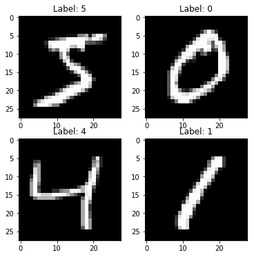

We’ll define network as a list of layers, each applied on top of previous one. In this setting, computing predictions and training becomes trivial.

network = []
network.append(Dense(X_train.shape[1],100))
network.append(ReLU())
network.append(Dense(100,200))
network.append(ReLU())
network.append(Dense(200,10))
 
def forward(network, X):
    # Compute activations of all network layers by applying them sequentially.
    # Return a list of activations for each layer. 
    
    activations = []
    input = X
    # Looping through each layer
    for l in network:
        activations.append(l.forward(input))
        # Updating input to last layer output
        input = activations[-1]
    
    assert len(activations) == len(network)
    return activations
 
def predict(network,X):
 
    # Compute network predictions. Returning indices of largest Logit probability
    logits = forward(network,X)[-1]
    return logits.argmax(axis=-1)
 
def train(network,X,y):
    # Train our network on a given batch of X and y.
    # We first need to run forward to get all layer activations.
    # Then we can run layer.backward going from last to first layer.
    # After we have called backward for all layers, all Dense layers have already made one gradient step.
    
    
    # Get the layer activations
    layer_activations = forward(network,X)
    layer_inputs = [X]+layer_activations  #layer_input[i] is an input for network[i]
    logits = layer_activations[-1]
    
    # Compute the loss and the initial gradient
    loss = softmax_crossentropy_with_logits(logits,y)
    loss_grad = grad_softmax_crossentropy_with_logits(logits,y)
    
    # Propagate gradients through the network
    # Reverse propogation as this is backprop
    for layer_index in range(len(network))[::-1]:
        layer = network[layer_index]
        
        loss_grad = layer.backward(layer_inputs[layer_index],loss_grad) #grad w.r.t. input, also weight updates
        
    return np.mean(loss)

TRAINING:

from tqdm import trange
 
def iterate_minibatches(inputs, targets, batchsize, shuffle=False):
 
    assert len(inputs) == len(targets)
 
    if shuffle:
 
        indices = np.random.permutation(len(inputs))
 
    for start_idx in trange(0, len(inputs) - batchsize + 1, batchsize):
 
        if shuffle:
 
            excerpt = indices[start_idx:start_idx + batchsize]
 
        else:
 
            excerpt = slice(start_idx, start_idx + batchsize)
 
        yield inputs[excerpt], targets[excerpt]
 
from IPython.display import clear_output
 
train_log = []
val_log = []
 
for epoch in range(25):    
 
	for x_batch,y_batch in iterate_minibatches (X_train,y_train,batchsize=32,shuffle=TrUe):
        train(network, x_batch,y_batch)
 
   train_log.append(np.mean(predict(network,X_train)==y_train))
   val_log.append(np.mean(predict(network,X_val)==y_val))
 
   clear_output()
   print("Epoch",epoch)
   print("Train accuracy:",train_log[-1])
   print("Val accuracy:",val_log[-1])
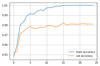
   plt.plot(train_log,label='train accuracy')
   plt.plot(val_log,label='val accuracy')
   plt.legend(loc='best')
   plt.grid()
   plt.show()