Humans don’t start their thinking from scratch every second. As you read this essay, you understand each word based on your understanding of previous words. You don’t throw everything away and start thinking from scratch again. Your thoughts have persistence.
Traditional neural networks can’t do this, and it seems like a major shortcoming. For example, imagine you want to classify what kind of event is happening at every point in a movie. It’s unclear how a traditional neural network could use its reasoning about previous events in the film to inform later ones.
Recurrent neural networks address this issue. They are networks with loops in them, allowing information to persist.
https://colah.github.io/posts/2015-08-Understanding-LSTMs/
A recurrent neural network has the structure of multiple feedforward neural networks with connections among their hidden units. Each layer on the RNN represents a distinct time step and the weights are shared across time.
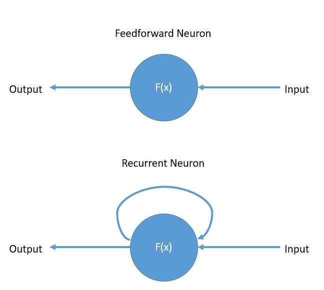
The basic difference between a feed forward neuron and a recurrent neuron is:
- The feed forward neuron has only connections from his input to his output.
- The recurrent neuron a connection from his output again to his input
- The major benefit is that with these connections the network is able to refer to last states and can therefore process arbitrary sequences of input.
These loops make recurrent neural networks seem kind of mysterious. However, if you think a bit more, it turns out that they aren’t all that different than a normal neural network. A recurrent neural network can be thought of as multiple copies of the same network, each passing a message to a successor:
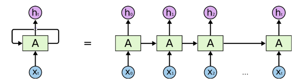
This chain-like nature reveals that recurrent neural networks are intimately related to sequences and lists. They’re the natural architecture of neural network to use for such data.
The RNN offers two major advantages:
- Store Information
- The recurrent network can use the feedback connection to store information over time in form of activations.
- Learn Sequential Data
- The RNN can handle sequential data of arbitrary length.

## Training of Recurrent Nets
The training of almost all networks is done by back-propagation, but with the recurrent connection it has to be adapted. This is simply done by unfolding the net like it is shown in figure:
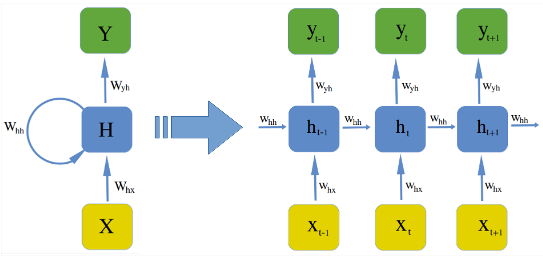
After unfolding, the network can be trained in the same way as a feed forward network with Backpropagation, except that each epoch has to run through each unfolded layer. The algorithm for recurrent nets is then called Backpropagation Through Time (BPTT).
https://www.deeplearningbook.org/contents/rnn.html
## Step by Step:
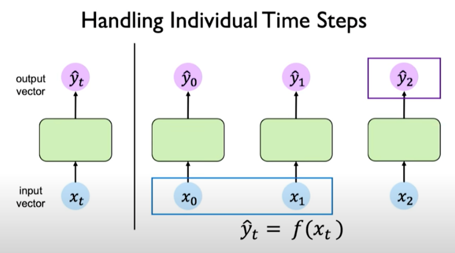
o support temporal information, we can treat individual time steps as isolated time steps.
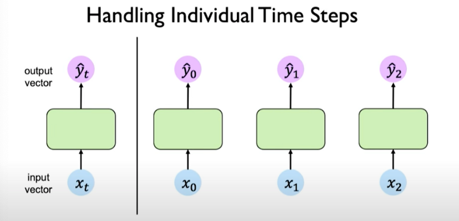
We still don’t have a notion of interconnectedness across time steps.
If we take the output of the last time step, the output is related to the inputs at the previous time steps. So the question is: how can we capture interdependence?
We need a way to related the network’s computations at a particular time step to its prior history and its memory of the computations from those prior time steps, passing information forward propagating it through time.
We can connect the computation of the network at different time steps via a recurrence relation. We can do this by introducing an internal memory or state, denoted as . This value is maintained time step to time step and can be passed forward across time. The idea for this state is to capture some notion of memory.
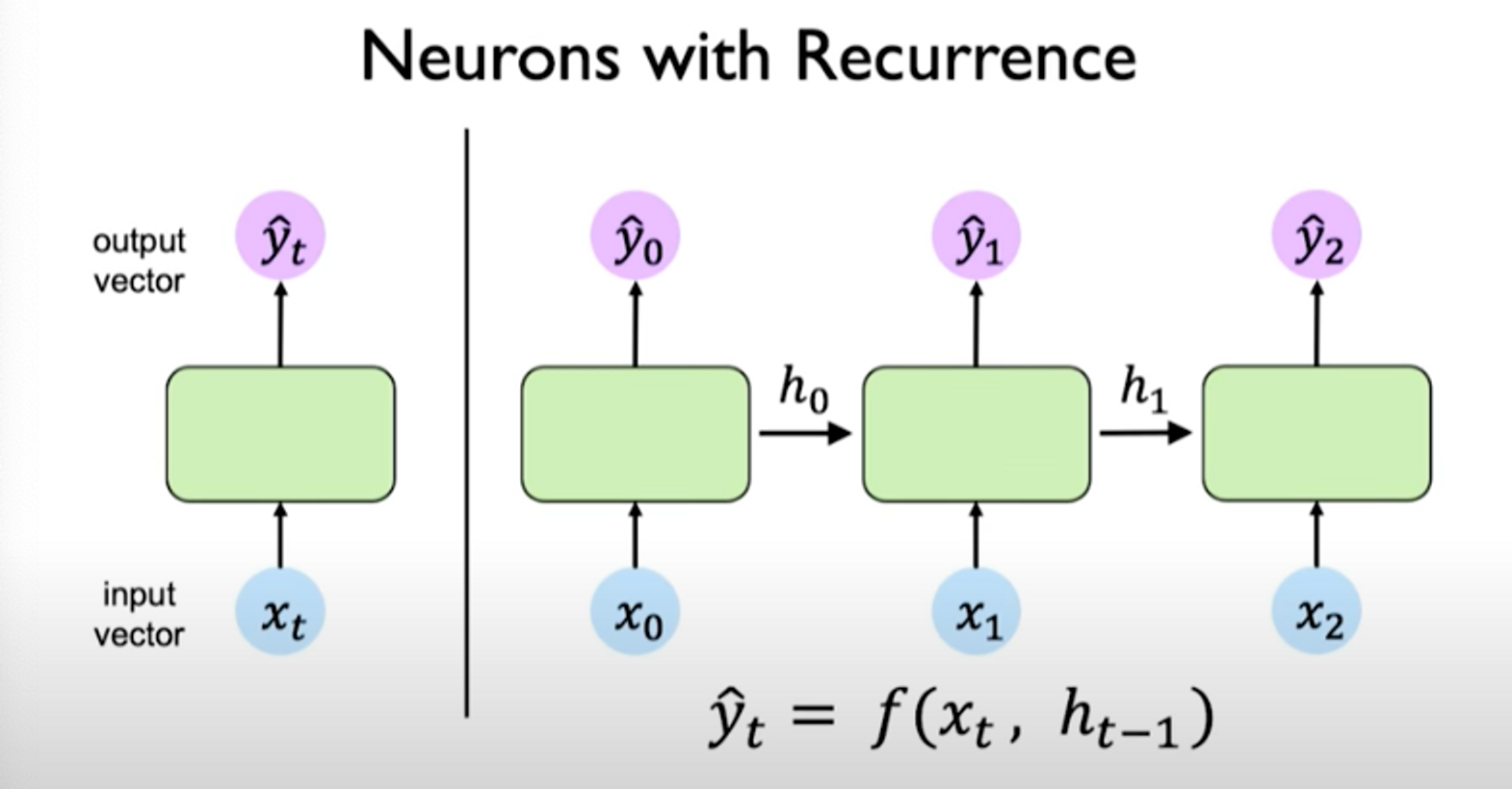
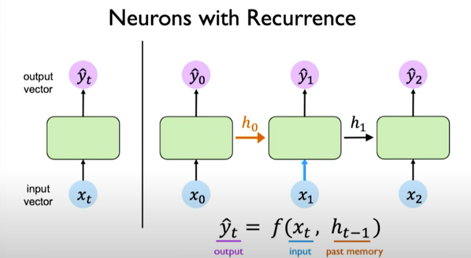
The output depends on the input as well as past memory. The past memory capture prior history of what has occurred previously in the sequence.
We can visualize these operations as follows:
left: recurrence relationship depicted via cycle right: individual time steps operations being unrolled and extended across time
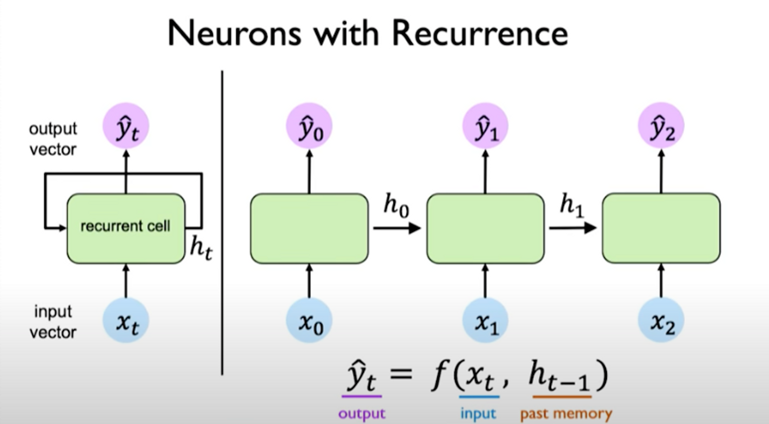
The hidden state is updated at each time step as the sequence is processed.
Essentially, a recurrence relation at every time step is applied to process the sequence:
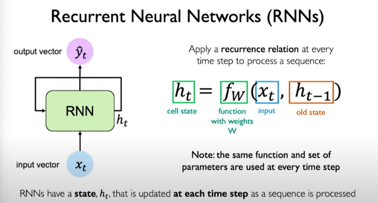
The set of weights learned is the same across all time steps that are considered in the sequence.
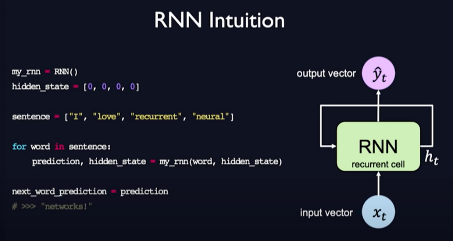
Here is a pseudocode example of RNNs to get an intuition of how it works:
The steps to update hidden state and output are shown below:
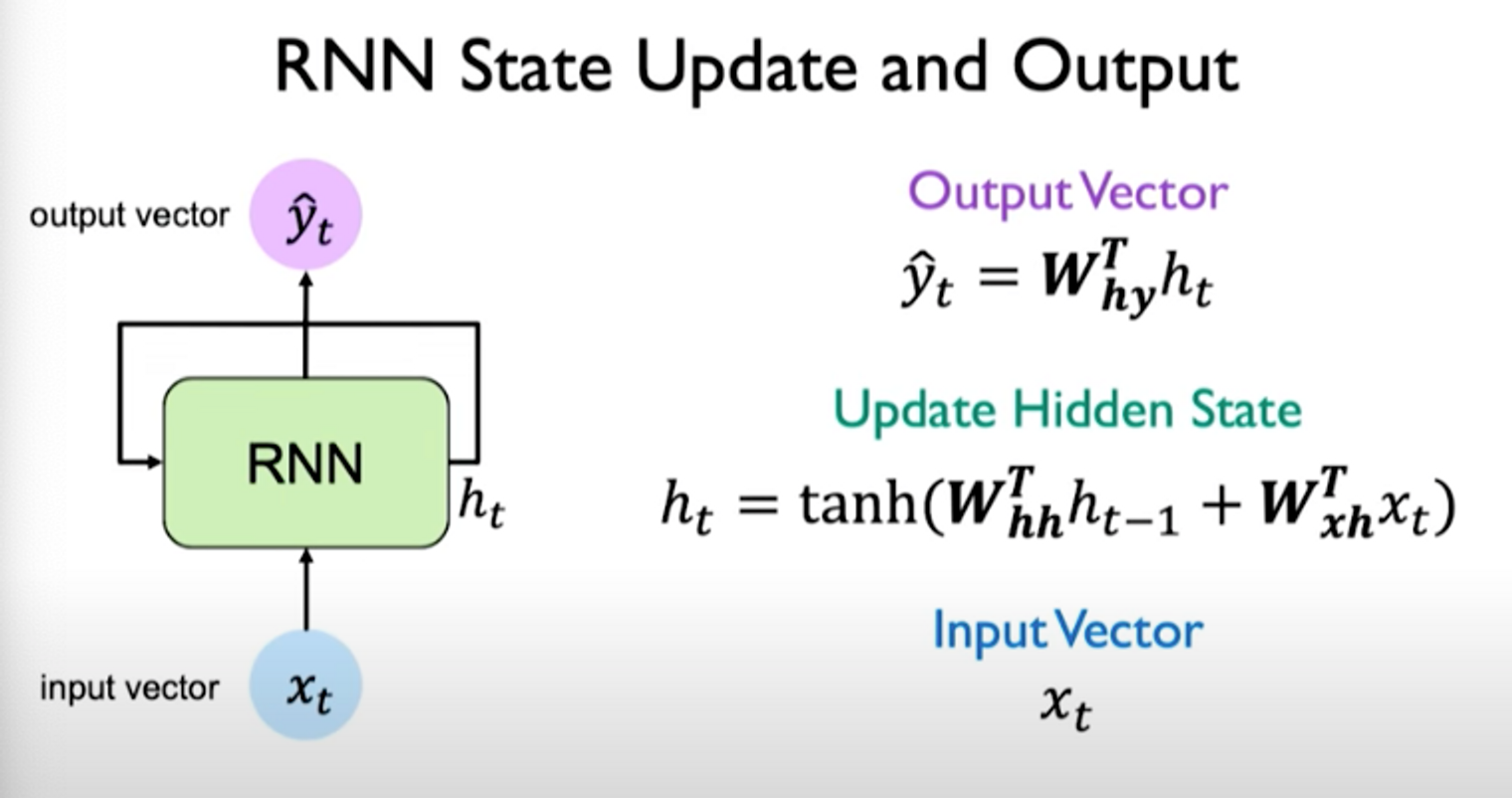
Note that there are independent weights matrices used for updating the hidden state. The output operation also uses a separate weight matrix multiplied by the hidden state. The operations are as follows:
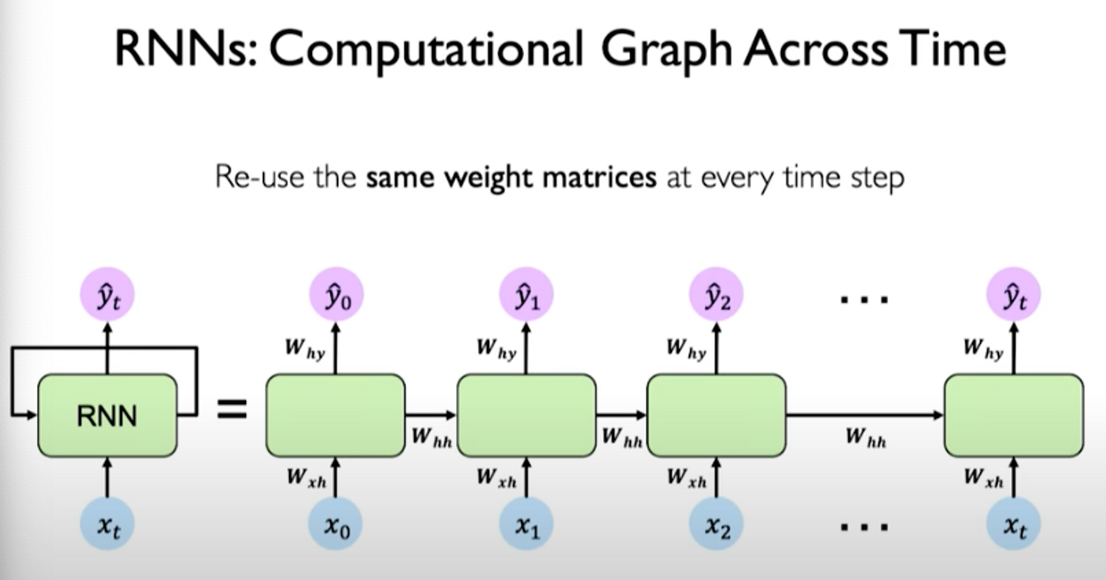
The computational graph looks as follows:
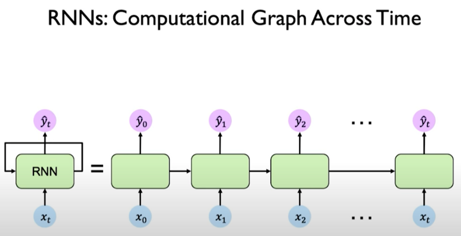
When we look at the exact components involved in the operations of an RNN, we notice that the same weight matrices are re-used at every time step.
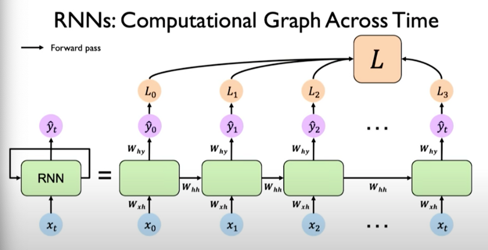
For training this network, we introduce a loss which can be calculated individually for each individual time step. It’s based on the output at that time step.
We can then generate a total sum loss by taking loss at every time step as summing them all together. So now when we make forward pass through the network, it outputs predictions which are used to generate losses and summed across individual time steps:
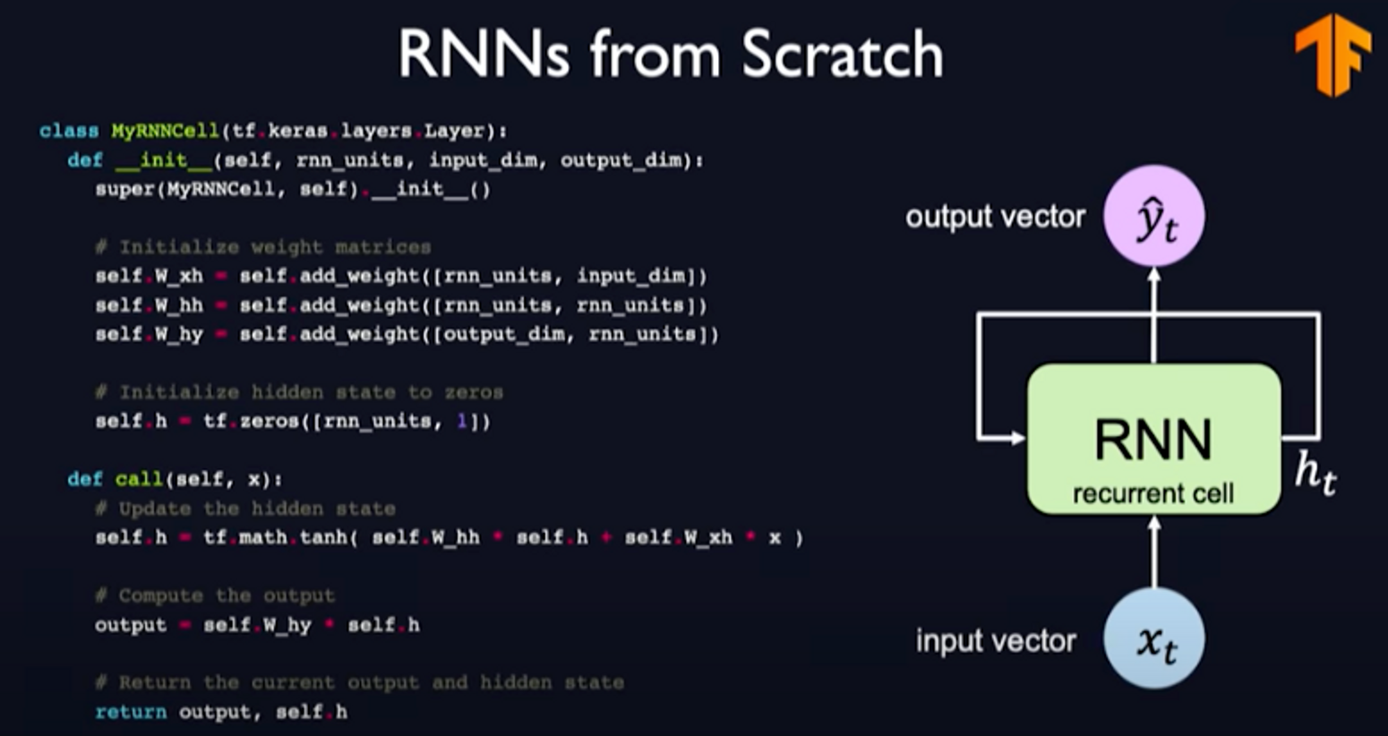
Implementing RNNs from scratch could look as follows:
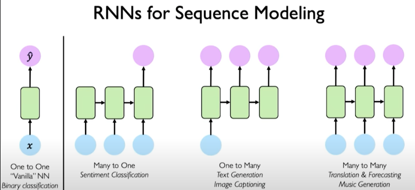
RNNs for sequence modeling
Here are some of the different ways RNNs can be used to solve different types of problems.
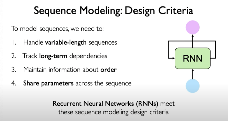
The design criteria for sequence modeling looks as follows:
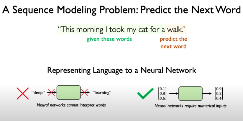
Predict the Next Word
Let’s look at how to use those specifications for a basic sequence modeling problem: predict the next word.
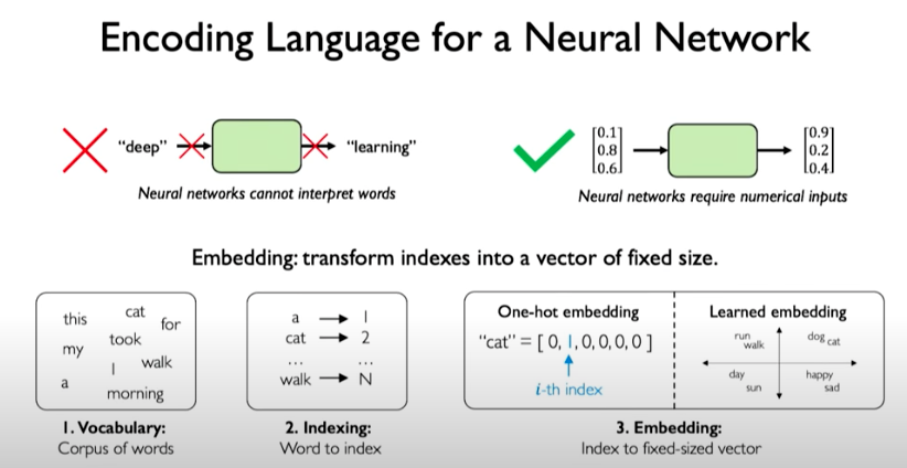
To make use of RNNs in a problem like predicting the next word, we need to represent inputs numerically.
One way to encode language for a neural network is called embeddings. Embeddings can be represented as sparse vectors called one-hot embeddings or embeddings learned using a machine learning model that capture the semantic similarity of words and that meaning is represented in some latent way through the vectors.
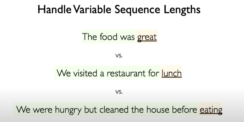
Our network should be able to handle variable sequence lengths.
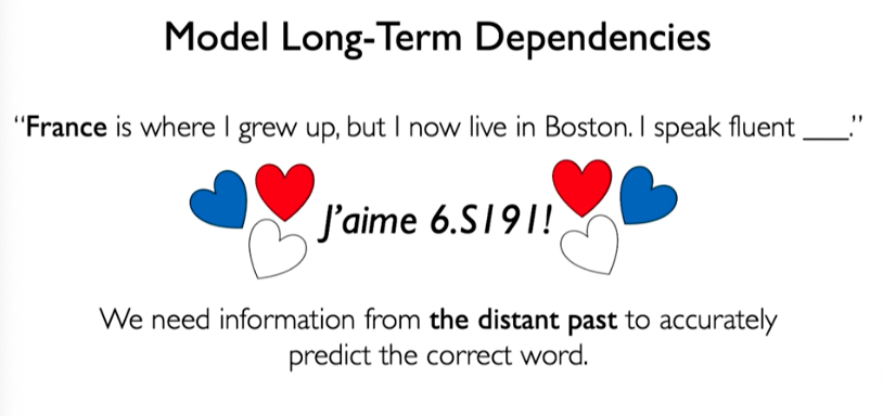
We also want to be able to capture long-term dependencies.
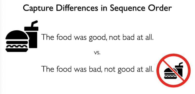
We want to also retain some sense of order to preserve meaning.
Backpropagation Through Time (BPTT)
BPTT is the algorithm for training this model. Recall what propagation in FF models does the following:
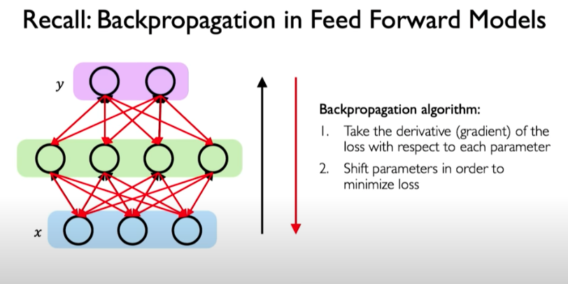
In RNNs, the forward pass involves going forward across time. We can backpropogate the errors individually across each time step and then across all time steps. In other words, errors flow backwards in time to the beginning of the sequence.
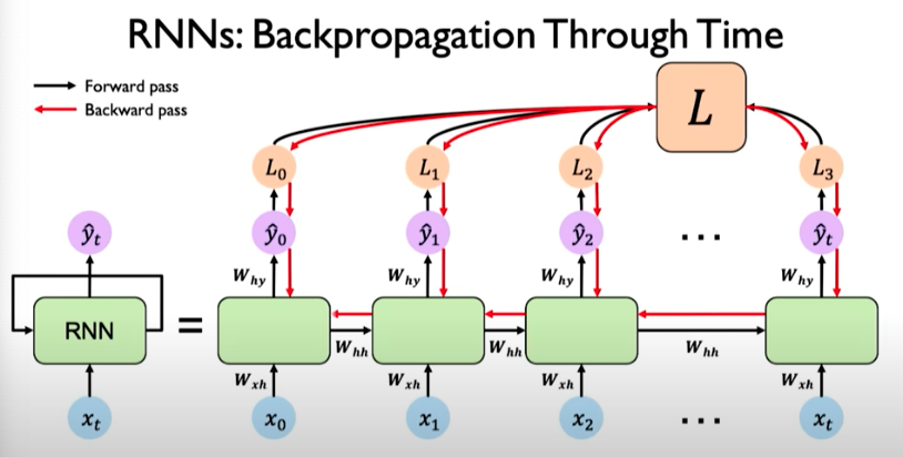
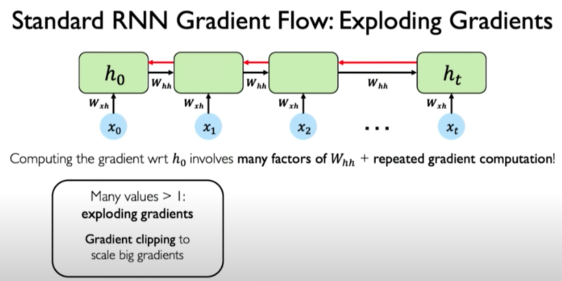
To compute the gradients it requires many matrix multiplications involving the weight matrix as well as repeated gradient computation. This repeated multiplication operation is problematic because gradients might explode during training in the situation where many values are much larger than 1.
A simple solution is called gradient clipping, where we trim the gradient values to scale back bigger gradients into a smaller value.
The opposite can also occur, where weight values are very small and this leads to vanishing gradients. It can be mitigated using the following three ways:
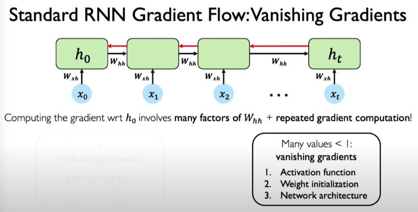
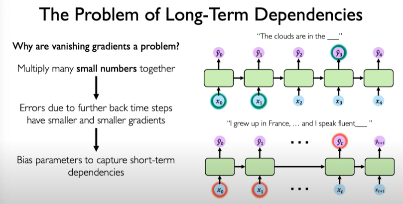
When we are multiplying many smaller numbers together, it could bias the model to potentially focus on short-term dependencies and effectively ignore the long-term dependencies.
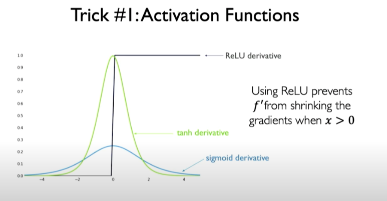
Trick #1: Activation Functions
Choose activation functions to prevent gradient from shrinking too dramatically. ReLU is a good choice because value of activation function are boosted to 1 when x > 0.
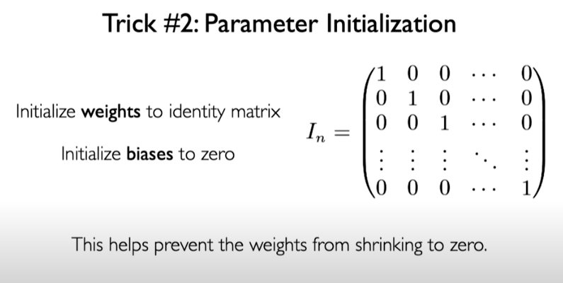
Trick #2: Parameter Initialization
We can initialize weight to identity matrix to prevent the weights from shrinking to zero.
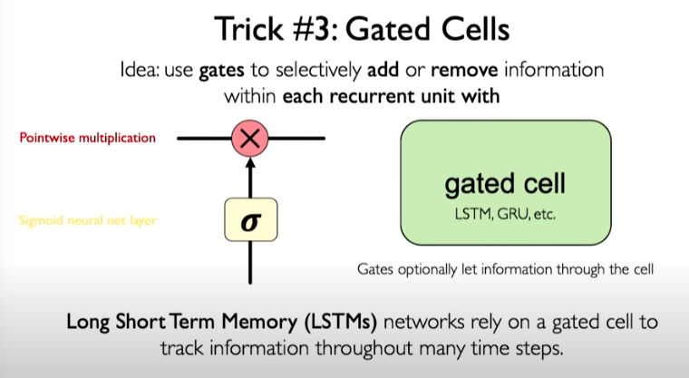
Trick #3: Gated Cells
A more robust solution is to use a more complex recurrent unit to track more effectively the long-term dependencies. Gates help to selectively add or remove information within each recurrent unit. One example is called LSTM.
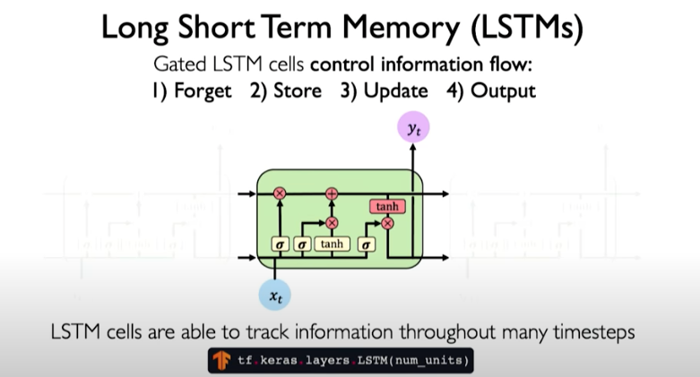
In LSTMs, there are many operations introduced to help control information flow.
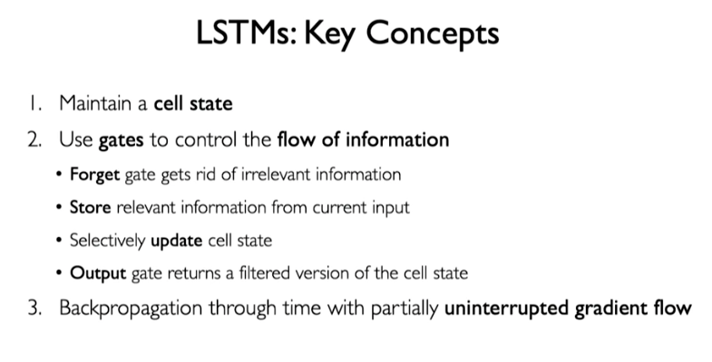
LSTMs: Key Concepts
RNN Applications & Limitations
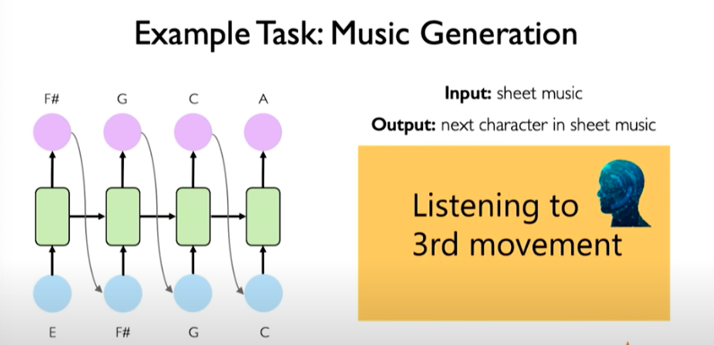
We can train a model to predict next musical note in sequence and generate brand new musical sequences. We can treat is a next time step prediction problem.
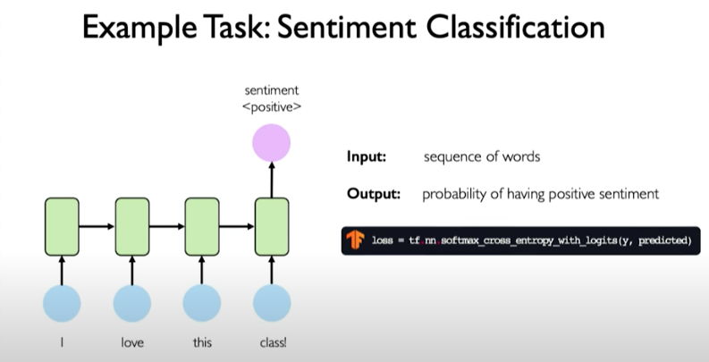
Another example task: sentiment classification where we are predicting a single output like the sentiment of a sentence.
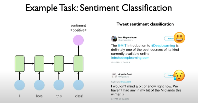
Example could be a tweet sentiment classification.
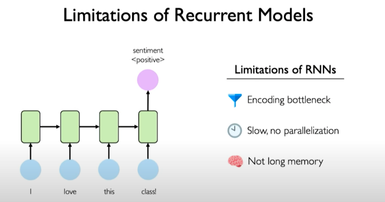
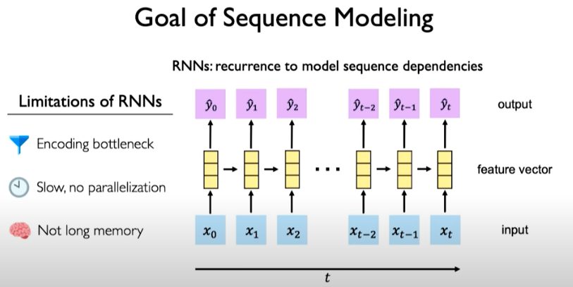
Limitation of Recurrent Models
RNNs have an encoding bottleneck because we need to take a lot of content and condense it to a representation that can predicted on. Information can be lost in the encoding operation.
RNNs are not efficient at all! They request information to processed sequentially. It makes them very inefficient on the modern GPU hardware.
Recurrent models don’t have high memory capacity and struggle with very long sequences, say the size of 1000 or 10000.
According to Alayrac et al. (2022), more recent architectures like Transformers, “improve modeling of long-range dependencies over RNN-based approaches, while significantly increasing the throughput of models and therefore the amount of data seen during training.”
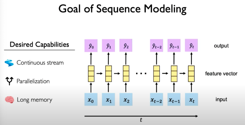
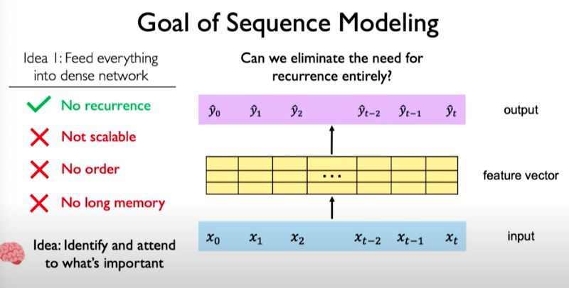
Goal of Sequence Modeling
The desired capabilities would be as follows: - Continuous stream of information that overcome the encoding bottleneck - Model should be parallelizable - Should be able to scale and support long memory
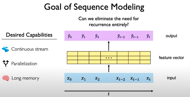
What if we can eliminate the need for recurrence entirely?
One way to do this is by squashing everything together. Concatenating those individual time steps such that we have one vector of input with data from all time points and feed it into a model to calculate some feature vector and then generate an output.
This approach however, limits us as follows:
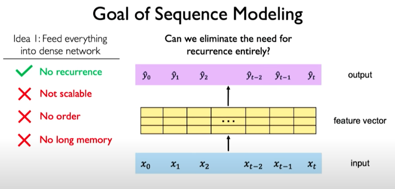
The other issue is that we don’t have a notion of what points in our sequence is important. This is the key idea behind the concept called attention that will be discussed next.
Attention is All You Need
Although the maths for attention mechanism could be daunting, the intuition behind it is simple.
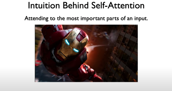
Given the image above, our brain is able to pickup that the character “iron man” is important.
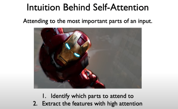
To perform this recognition, you first identify which parts to attend to, which is similar to a search problem.
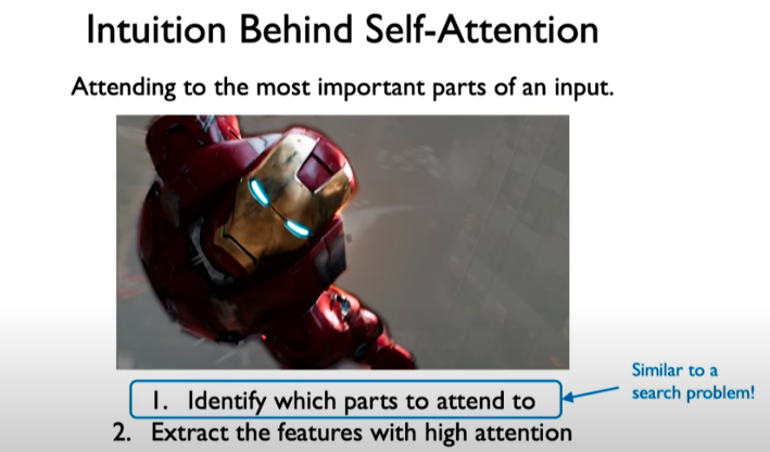
To explain search, let’s explain a simple example of finding YouTube videos.
First we input a query. For every video in the database, some key information is extracted (e.g., title). To perform the search, you can compute the overlap between keys and queries. For every check, we ask how similar is that key to the query.
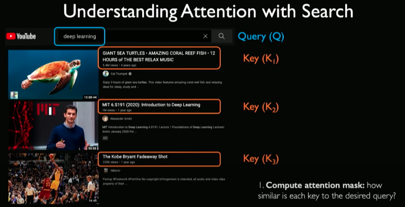
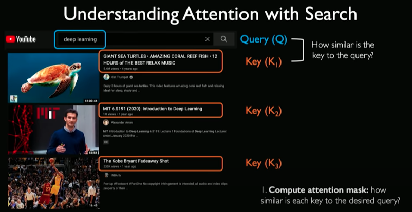
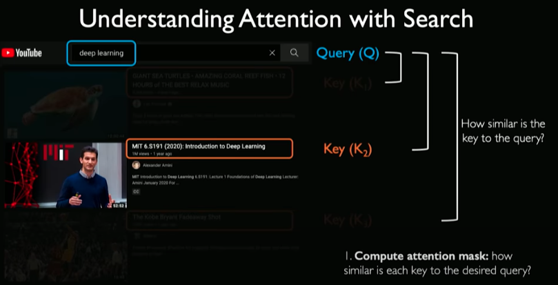
So essentially we are computing an attention mask measuring how similar each of these keys are to the query.
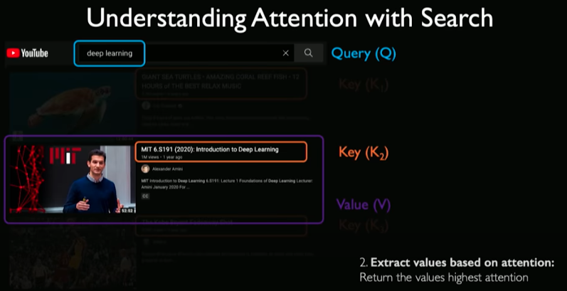
The final step is to extract the information (the video itself) we care about based on the computation. This is referred to as the value.
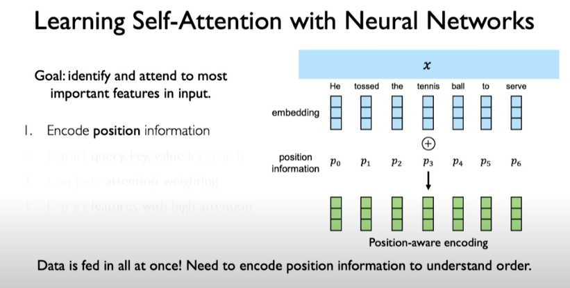
With this new way of analyzing and processing sequences, we avoid the need to process the words in the sentences individually.
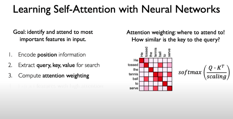
We can encode position information using position-aware encoding.
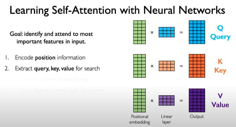
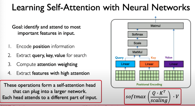
We then need a mechanism to identify and attend to the most important features in the input. Here we are doing self-attention meaning we are only operating on the input itself. To produce the query, key, and value representations, we can do the following:
Then we take those three representations and compute the attention weighting. This can be done by computing pairwise similarity between each query and key, similar to the example we showed before related to the video search. We do this applying dot product operation which can then be applied to matrices.
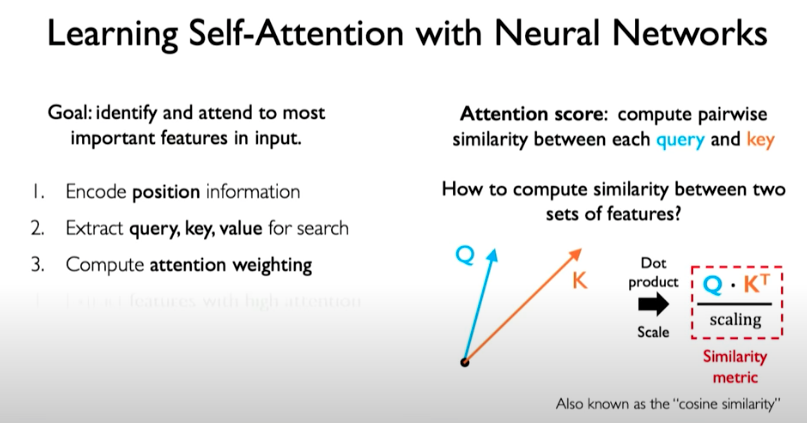
We now have a similar metric that captures the similarity between the query matrix and the key matrix.
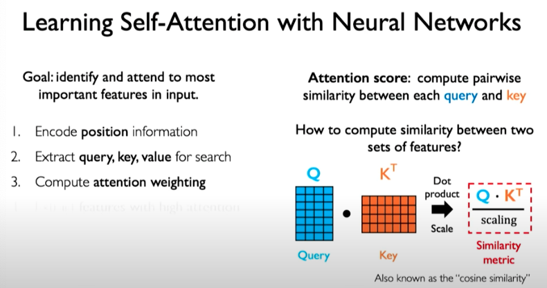
With an example, this operation looks as follows. We perform dot product, then scale, and then apply softmax operation, which squashes values to fall between 0 and 1.
The output matrix reflect the relationship between the components of our input to each other. We can see that words related to each other have a higher weight, a higher attention. The matrix is called attention weighting.
The final step is to use this matrix to extract features with high attention. We do this by taking attention weighting matrix and multiplying by value matrix to get a transformed version of the value matrix. The final output reflects the features that correspond to high attention.
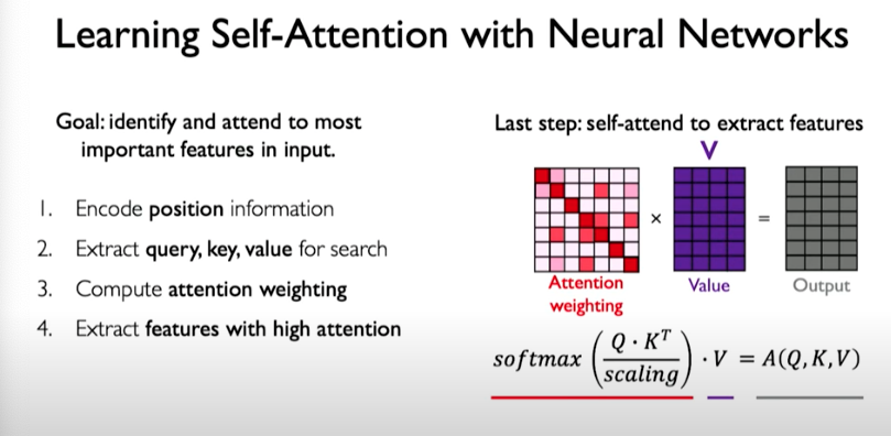
In summary:
We can do this operation multiple times. In other words, we can implement different attention heads that attend to different things in the input.
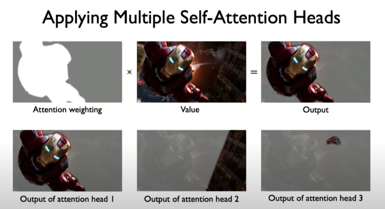
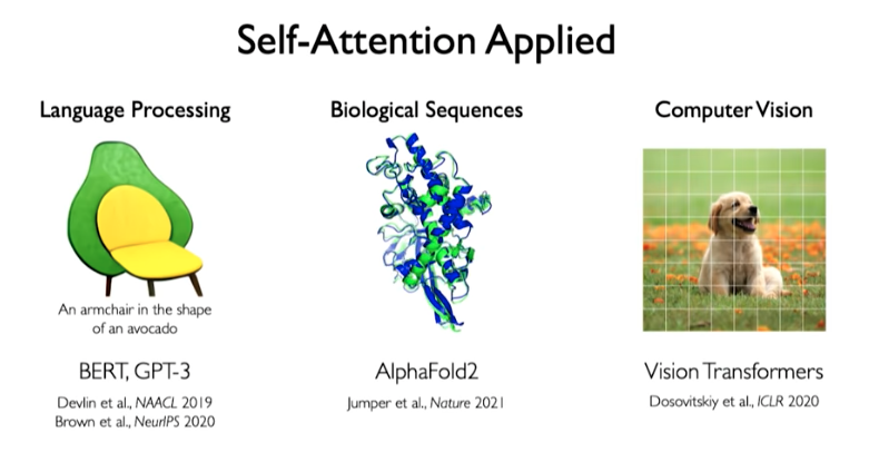
Self-Attention Applied
The idea of self-attention is now being applied to advance machine learning models in many areas such as language processing, biological sequences, and compute vision.
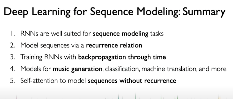
Deep Learning for Sequence Modeling: Summary
References: - Generating sequences with recurrent neural networks - Attention Is All You Need - NOTION_PAGE:71fb3ba2-a24f-4b6c-8cc7-7281fc19cfab
https://distill.pub/2016/augmented-rnns/ https://www.analyticsvidhya.com/blog/2021/06/a-visual-guide-to-recurrent-neural-networks/ https://wiki.pathmind.com/lstm